Global overview Power Pivot: The basics.

Introduction
In general Power Pivot is a datawarehouse engine within Excel.  If you use it with financial data of your company, you will get more insight in what is happening in our company. You can get insight from different perspectives. With this insight you can look how you can do it better. A Power Pivot sheet will contain the following components:

• Datasets
• Measures
• Relationships between datasets
• Time dimension dataset
• PivotTables and PivotCharts

Datasets

Every Power Pivot sheet can contain one or more datasets. For instance you have a dataset for your Debtors and a dataset for your Invoices.  Dataset Debtors will contain all related Debtor information like, Debtor code, Country, State, Sector etc. Useful information is data which can be used filters or group by calculations etc. For instance, country of a debtor can be used to show revenue per country. Phone number is not useful because it is unique for one customer. Revenue per phone number is the same as the revenue per debtor.  Datasets are defined in the Power Pivot Window. The Power Pivot Window button is part of the Power Pivot tab of the ribbon.

 

Example of the dataset debtors:

Example of the dataset Invoices: 

Dataset Invoices: Click to enlarge

Measures
In every dataset you can define measures. A measure is a formula that is created specifically for numeric data that you want to summarize or analyze in a PivotTable or PivotChart. Measures can be based on standard aggregation functions, such as COUNT, AVERAGE or SUM, or you can define your own formula by using DAX.
Example of measures on the Invoices dataset, like Invoices, Invoices per Customer, Invoiced customers, Average Invoice amount  etc.

Defined measures will be available in the Power Pivot field list and can be recognized by the calculator symbol.

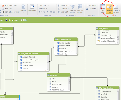
Relationships between datasets  Datasets can be linked to each other by creating a relationship between the tables. The relationship establishes how the data in the two tables should be correlated. For example, a Debtor table and an Invoice table can be related in order to show the customer name that is associated with each order. After you have defined a relationship between tables in the Power Pivot window, you will be able to filter data by using related columns, lookup values in related tables, and integrate columns from multiple tables in a PivotTable. To understand with related columns can be used, you need to look to the defined relations. Open the Power Pivot window and press on the Diagram View button in the ribbon.

Diagram View: Click to enlarge

Time dimension dataset
To make use of the powerful Time intelligent functions it is recommended to create a separate related time table. To create such a table read: http://www.keepitsimpleandfast.com/2012/09/script-to-generate-time-dimension-table.html  The TimeDimension table contains characteristics of all days. For instance the day 24 may 2013. Some examples of the characteristics of this day: Year: 2013, Month: 5, It’s a Friday, Quarter 2, ISO week number: 21 All these different characters can be used in your pivots. Link your time dimension table to the date columns on your other datasets. For instance link Invoice date of your Invoice table to the date column.

This enables you to build revenue reports per week, month etc.
PivotTables and PivotChartsAfter having defined datasets, relationships, a date time table and measures, we can start building the reports.  Select the Power Pivot Tab in the ribbon, Select PivotTable and select what you want to insert.

You will get the Power Pivot field list which you need to use to define your chart. 

This will result in next chart:

Add a second chart or pivot to the same sheet. If you change slicer values of the previous chart, the added pivot or chart does not change. You need to link the added chart or pivot to the slicer. To do these select the added chart or pivot. Select the Pivot Table Tools, Options tab. Select Insert Slicer, Slicer Connections. You will get a list of all slicers. Select the slicer of the current sheet. The slicer is now active on both charts\pivots. You can check this by changing the slicer values.